Graphs

Introduction

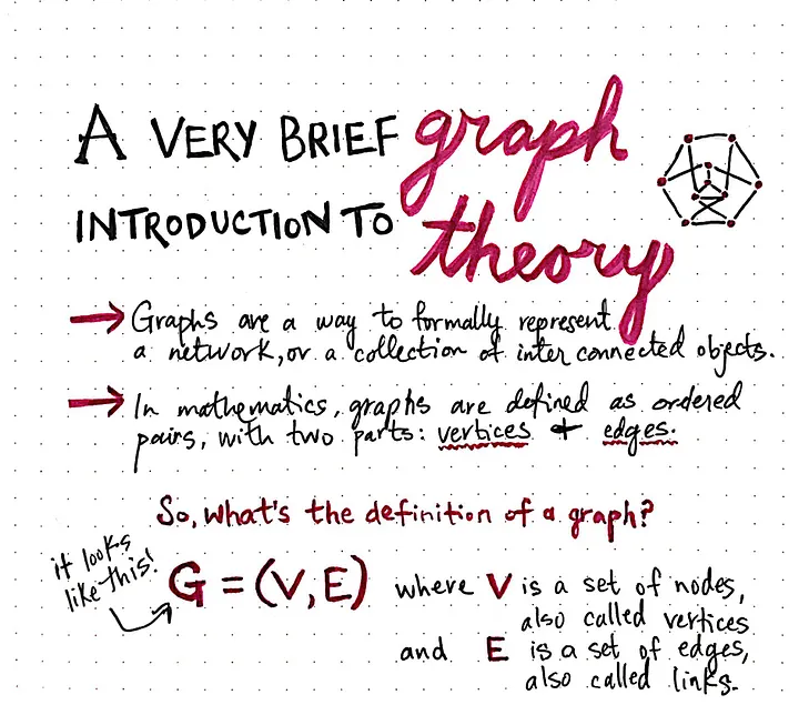
In mathematics and computer science, Graph Theory is the study of graphs, which are mathematical structures used to model pairwise relations between objects. A graph in this context is made up of vertices (also called nodes or points) which are connected by edges (also called arcs, links, or lines). A distinction is made between undirected graphs, where edges link two vertices symmetrically, and directed graphs, where edges link two vertices asymmetrically. Graphs are one of the principal objects of study in discrete mathematics.

In General Graph is a set of points, called vertices together with a collection of lines called edges.

Basic Concepts

Node and Edge

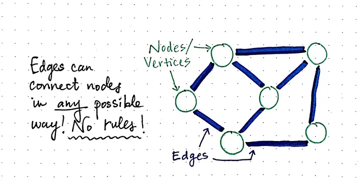
• A Node (vertex) is the basic unit in a graph, it represents an object, state or point in the system
• An edge is a connection between two nodes, it represents a relationship or transition between two objects(nodes), a road between two cities, or an action that changes one state to another
• In AI search, you usually think of nodes as states and edges as actions or transitions that take you from one state to another, possibly with a cost attached (making the graph weighted).

Directed vs Undirected Graphs

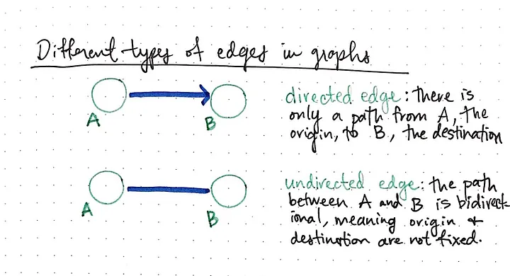
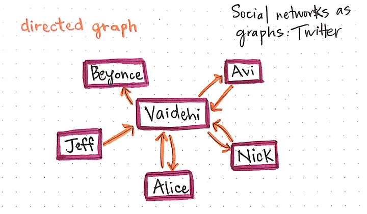
• In a directed graph (digraph), each edge has a direction (often drawn as an arrow). An edge from A to B only lets you go from A to B, not necessarily back; the relationship is asymmetric, like “follows” on social media or a one‑way street.

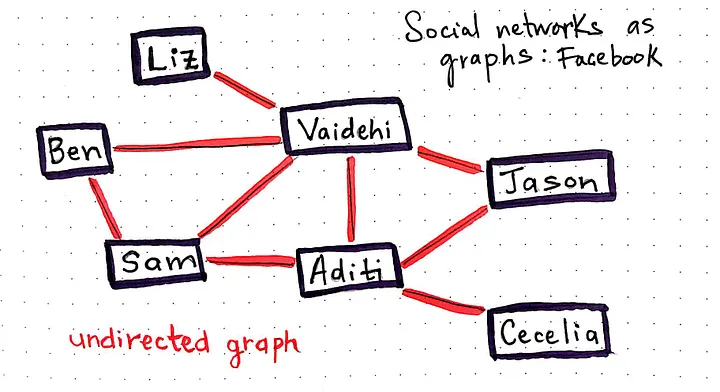
• In an undirected graph, edges have no direction. If there is an edge between node A and node B, you can go from A to B and from B to A in the same way. The relationship is symmetric, like “friends with” or a two‑way road.

• In AI search, undirected graphs often model reversible actions (you can undo a move), while directed graphs model irreversible or one‑way transitions (e.g., state changes in a game where certain moves cannot be reversed).

Weighted vs. unweighted graphs

A graph can be divided into weighted and unweighted based on weight

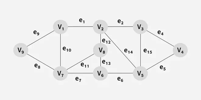
• In an unweighted graph, all edges are treated as equal: there is no “cost” or “value” on the edges, only the presence or absence of a connection. Paths are usually compared by how many edges (hops) they use, so the “shortest path” means the one with fewest steps

  • AI Context: Breadth-First Search (BFS) operates here. You just want the shortest _number of steps

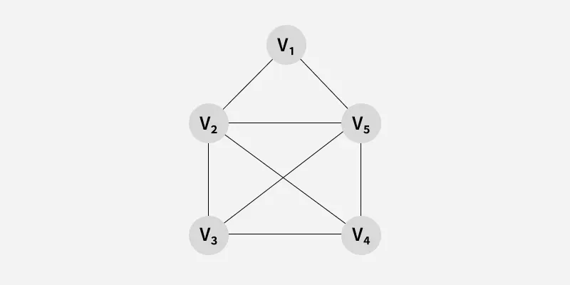
• In a weighted graph, each edge has a number (a weight) attached, such as distance, time, or cost. The shortest path is then the one with the smallest total weight, not necessarily the fewest edges. Algorithms like Dijkstra and Uniform Cost Search rely on these weights

  • AI Context: Crucial for A and Dijkstra._* The distance in miles between cities; The time to traverse a corridor in a video game (mud = high weight, road = low weight).

In General, Unweighted graphs assume all edges equal, ideal for basic connectivity checks. Weighted graphs assign values (e.g., distance, cost) to edges, enabling optimizations like shortest paths in GPS apps. Weights add realism for real-world modeling but increase computational complexity

Adjacency and degree

Adjacency means two vertices (nodes) are directly connected by an edge. In an undirected graph, if there is an edge between uu and vv, both are adjacent to each other. In a directed graph, we say vv is adjacent from uu if there is an edge from uu to vv.

Degree of a vertex is the number of edges connected to it. In an undirected graph, it is simply the number of neighbors (adjacent vertices). In a directed graph, we often split this into in‑degree (how many edges come in) and out‑degree (how many edges go out) Degree:

• Undirected: Number of edges connected to the node.
• Directed:
  • In-degree: Number of edges entering the node.
  • Out-degree: Number of edges leaving the node.
• AI Context: Branching Factor. In search, the out-degree dictates how many new states the algorithm must evaluate at each step. High branching factor = computationally expensive search.

Paths and Cycles

• Path: is a sequence of vertices connected by edges, where you start at one vertex and end at another, and you do not repeat any vertex (and so implicitly no edge is repeated either). In AI search, a path often represents a valid sequence of actions from a start state to a goal state.

  • AI Context: The solution found by the search algorithm (e.g., “Turn Left, Go Straight, Turn Right”).

• Cycle: is a special kind of path that starts and ends at the same vertex, with no other vertex repeated; it “loops” back to the start. In AI, a cycle in the state‑space graph means you can come back to a state you’ve visited before, which can cause infinite loops if the search is not careful.

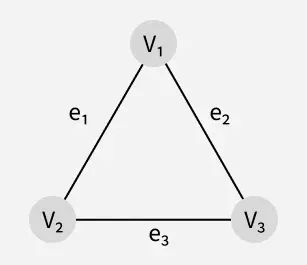
  • AI Context: The Nemesis of AI Search. If a graph has cycles (e.g., moving back and forth between two rooms), a naive search algorithm will get stuck in an infinite loop. Cycle Detection (keeping a “Visited” set) is mandatory in most AI algorithms.

Connected vs. Disconnected Graphs

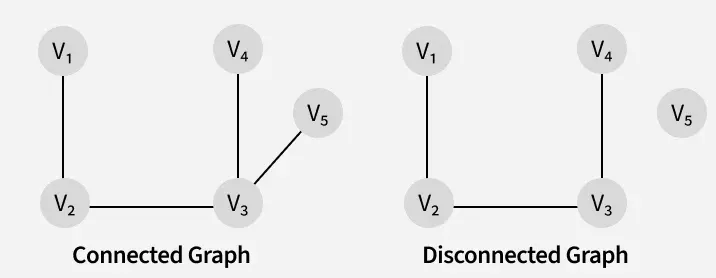
A connected graph is one where you can reach any node from any other node by following some path. In other words, between every pair of vertices there exists at least one path.

A disconnected graph is one where at least two vertices cannot be reached from each other; there is no path between them. Such a graph breaks into two or more separate pieces, each internally connected; each piece is called a connected component

In AI search, if your state‑space graph is disconnected, it means some states are completely unreachable from the start state, so they will never be explored by BFS/DFS/etc. starting from that initial node

Trees as Special Graphs

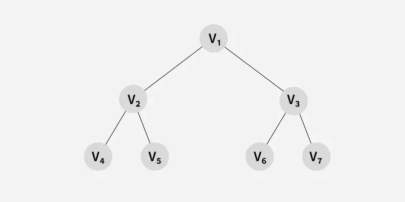
• A tree is a special kind of graph that is connected and acyclic, meaning:
  • It is connected: there is a path between any two nodes.
  • It has no cycles: no path loops back to a node already visited.
• Key properties of trees:
  • There is exactly one unique path between every pair of nodes.
  • For n vertices, a tree has exactly n−1 edges.
  • If you remove any edge, the graph becomes disconnected; add any edge and you create a cycle.
• In AI search, trees often model state spaces where each transition leads to a new state without cycles (like a game tree or simple search tree), while general graphs allow cycles and multiple paths between states.

Connected Components

• A connected component of an undirected graph is a maximal set of nodes such that every node in the set can reach every other node in that set via some path, and there are no edges connecting this set to any node outside it.

• In plain terms:

  • A connected component is a “piece” of the graph that is internally connected; you can walk from any node in that piece to any other node in the same piece, but you cannot go to nodes in another piece.

  • A graph can have one connected component (if it is fully connected) or many (if it is disconnected), and all components together form a partition of all the vertices.

  • Algorithms like DFS or BFS identify components in O(∣V∣+∣E∣) time.

• In AI search, connected components are useful because if your start state is in one component, the search can only reach states in that same component; states in other components are unreachable from the start.

Directed Acyclic Graphs (DAGs)

• A DAG (directed acyclic graph) is a directed graph with no directed cycles, meaning:

  • Edges have direction (arrows), and

  • You cannot follow the arrows and return to the same node you started from.

• Because of this, DAGs can be topologically ordered: nodes can be arranged in a sequence such that every edge goes from an earlier node to a later one. This makes DAGs perfect for modeling dependencies such as task schedules, pipelines, or causal relationships.

• Search Efficiency: Finding shortest paths in a DAG is $O(V+E)$, faster than Dijkstra, because the lack of cycles removes the need for complex priority queue updates.

• In AI and CS, DAGs are used in things like task‑dependency graphs (e.g., build pipelines, data‑flow graphs) and Bayesian/causal networks, where edges represent “this node must happen before that one” or “this variable causally affects that one.”

Adjacency List Representation

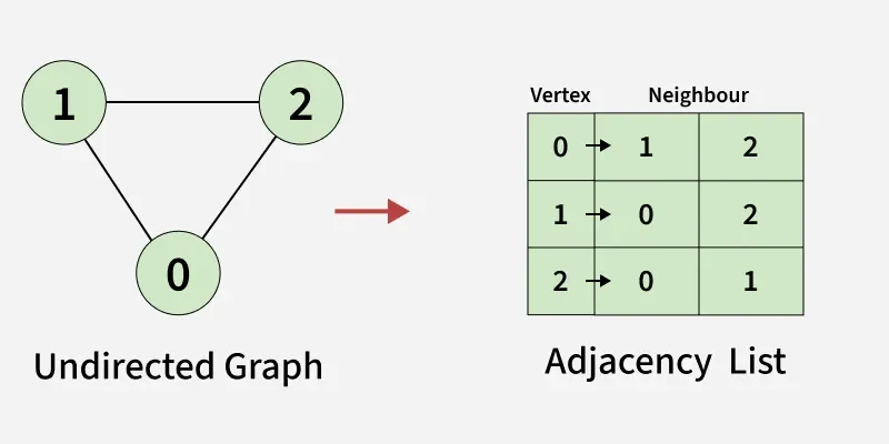
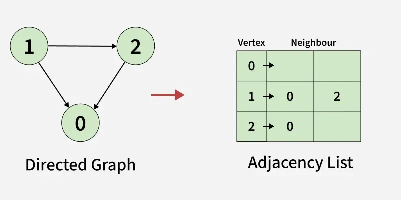
An array of Lists is used to store edges between two vertices. The size of array is equal to the number of vertices (i.e, n). Each index in this array represents a specific vertex in the graph. The entry at the index i of the array contains a linked list containing the vertices that are adjacent to vertex i. Let’s assume there are n vertices in the graph So, create an array of list of size n as adjList[n].

• adjList[0] will have all the nodes which are connected (neighbour) to vertex 0.

• adjList[1] will have all the nodes which are connected (neighbour) to vertex 1 and so on.

• Practical features:

  • Very space‑efficient for sparse graphs (few edges) because you store only existing edges.

  • Easy to iterate over neighbors of a node, which is exactly what BFS/DFS and many AI search algorithms do when they expand a state.

  • Space: $O(\mid V\mid +\mid E\mid )$ , efficient for sparse graphs.

  • Time to check adjacency: $O(deg(v))$.

• When to use in AI search:

  • Ideal for state‑space graphs where the number of actions per state is small compared to the total number of states (most of the matrix would be zeros).

Representation of Undirected Graph as Adjacency list:

def createGraph(V, edges):
    adj = [[] for _ in range(V)]
 
    # Add each edge to the adjacency list
    for it in edges:
        u = it[0]
        v = it[1]
        adj[u].append(v)
        
         # since the graph is undirected
        adj[v].append(u)
    return adj
  
 
if __name__ == "__main__":
    V = 3
 
    # List of edges (u, v)
    edges = [[0, 1], [0, 2], [1, 2]]
 
    # Build the graph using edges
    adj = createGraph(V, edges)
 
    print("Adjacency List Representation:")
    for i in range(V):
        
        # Print the vertex
        print(f"{i}:", end=" ")
        for j in adj[i]:
            
            # Print its adjacent
            print(j, end=" ")
        print()

output

Adjacency List Representation:
0: 1 2 
1: 0 2 
2: 0 1

Representation of Directed Graph as Adjacency list:

def createGraph(V, edges):
    adj = [[] for _ in range(V)]
 
    # Add each edge to the adjacency list
    for it in edges:
        u = it[0]
        v = it[1]
        adj[u].append(v)
 
    return adj
  
 
if __name__ == "__main__":
    V = 3
 
    # List of edges (u, v)
    edges = [[1, 0], [1, 2], [2, 0]]
 
    # Build the graph using edges
    adj = createGraph(V, edges)
 
    print("Adjacency List Representation:")
    for i in range(V):
        
        # Print the vertex
        print(f"{i}:", end=" ")
        for j in adj[i]:
            
            # Print its adjacent
            print(j, end=" ")
        print()

output

Adjacency List Representation:
0: 
1: 0 2 
2: 0

Adjacency Matrix Representation

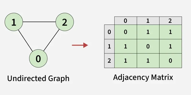
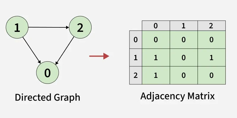
An adjacency matrix is a way of representing a graph as a boolean matrix of (0’s and 1’s).

Let’s assume there are n vertices in the graph So, create a 2D matrix adjMat[n][n] having dimension n x n.

• If there is an edge from vertex i to j, mark adjMat[i][j] as 1.

• If there is no edge from vertex i to j, mark adjMat[i][j] as 0.

• Practical features:

  • Very fast to check if an edge exists between two nodes (just look up $A[i][j]$ in $O(1)$.

  • Less space‑efficient for sparse graphs, because you allocate $V^2$ entries even if most are empty.

• When to use in AI search:

  • Useful when the graph is dense (many edges), or when you frequently need to check “is there an edge between these two states?”, or when the number of nodes is small (e.g., tiny puzzle graphs).

Representation of Undirected Graph as Adjacency Matrix:

def createGraph(V, edges):
    mat = [[0 for _ in range(V)] for _ in range(V)]
 
    # Add each edge to the adjacency matrix
    for it in edges:
        u = it[0]
        v = it[1]
        mat[u][v] = 1
        
         # since the graph is undirected
        mat[v][u] = 1 
    return mat
 
if __name__ == "__main__":
    V = 3
 
    # List of edges (u, v)
    edges = [[0, 1], [0, 2], [1, 2]]
 
    # Build the graph using edges
    mat = createGraph(V, edges)
 
    print("Adjacency Matrix Representation:")
    for i in range(V):
        for j in range(V):
            print(mat[i][j], end=" ")
        print()

output

Adjacency Matrix Representation:
0 1 1 
1 0 1 
1 1 0

Representation of Directed Graph as Adjacency Matrix:

def createGraph(V, edges):
    mat = [[0 for _ in range(V)] for _ in range(V)]
 
    # Add each edge to the adjacency matrix
    for it in edges:
        u = it[0]
        v = it[1]
        mat[u][v] = 1
 
    return mat
 
if __name__ == "__main__":
    V = 3
 
    # List of edges (u, v)
    edges = [[1, 0], [2, 0], [1, 2]]
 
    # Build the graph using edges
    mat = createGraph(V, edges)
 
    print("Adjacency Matrix Representation:")
    for i in range(V):
        for j in range(V):
            print(mat[i][j], end=" ")
        print()

output

Adjacency Matrix Representation:
0 0 0 
1 0 1 
1 0 0

Choosing Lists vs. Matrices for AI Search

Use adjacency list when:

• The graph is sparse (few edges compared to the number of nodes), which is very common in AI state spaces (e.g., mazes, grids, puzzles, planning problems).

• You mainly care about expanding a node’s neighbors (like in BFS, DFS, Uniform Cost, A*), where lists let you iterate quickly over only real neighbors.

• Space efficiency matters, since adjacency lists store only existing edges and therefore use much less memory for large, sparse graphs.

Use adjacency matrix when:

• The graph is dense (many edges, almost all pairs connected) or small (e.g., a tiny puzzle state space), so the $V\times V$ matrix is manageable.

• You frequently need to check very quickly whether an edge exists between two nodes (a simple $O(1)$ lookup), which can be useful in some advanced preprocessing or bookkeeping steps.

• You are doing algorithms that work nicely on the matrix form (like all‑pairs shortest paths), but this is less typical in basic AI search.

In AI search practice:

• Adjacency list is the default choice for most search problems (BFS, DFS, UCS, A* on mazes, grid‑worlds, 8‑puzzle, etc.) because it combines low memory and fast neighbor traversal.

• Reserve adjacency matrix mainly for very small graphs or special cases where dense connectivity and fast “is there an edge?” checks are more important than space usage.

Criteria	Adjacency List	Adjacency Matrix
Graph Type	Sparse Graphs (Few edges). Example: Real-world road networks where each intersection connects to 3-4 others.	Dense Graphs (Many edges). Example: A fully connected social network graph.
Memory	Excellent. Only stores existing edges.	Terrible for sparse. Wastes massive memory storing zeros.
Speed: Find All Neighbors	Fast ($O(Outdegree)$). Crucial for expanding a node in A* or BFS. You just iterate the list.	Slow ($O(V)$). Must scan the entire row to find non-zero entries.
Speed: Check Specific Edge	Slow ($O(Outdegree)$). Must search the list.	Instant ($O(1)$). Matrix[u][v] lookup.
AI Search Use Case	Pathfinding (A, Dijkstra, BFS, DFS).* This is the default choice for almost all AI state-space search. The search algorithm must expand children quickly.	Local Search / CSP / Neural Nets. When the graph is small but fully connected, or when you need to check adjacency between any two states instantly (e.g., checking if two queens attack in N-Queens).

Related

• DSA MOC — Full map of DSA topics
• Binary Search — Search on sorted/monotonic spaces (used in graph algorithms)
• Recursion — DFS is inherently recursive; call stack powers graph traversal
• Sorting Basics — Sorting before search; topological sort on DAGs
• Stacks, Queues and Monotonicity — BFS uses queues; monotonic stacks for next-element problems on graphs
• Two Pointers — Traversal patterns on arrays mirror graph traversal logic
• AI Agents — State-space search is fundamental to intelligent agents